Support Vector Machines
We will be analyzing the famous iris data set!
The Data
We will be using the famous Iris flower data set.
The Iris flower data set or Fisher’s Iris data set is a multivariate data set introduced by Sir Ronald Fisher in the 1936 as an example of discriminant analysis.
The data set consists of 50 samples from each of three species of Iris (Iris setosa, Iris virginica and Iris versicolor), so 150 total samples. Four features were measured from each sample: the length and the width of the sepals and petals, in centimeters.
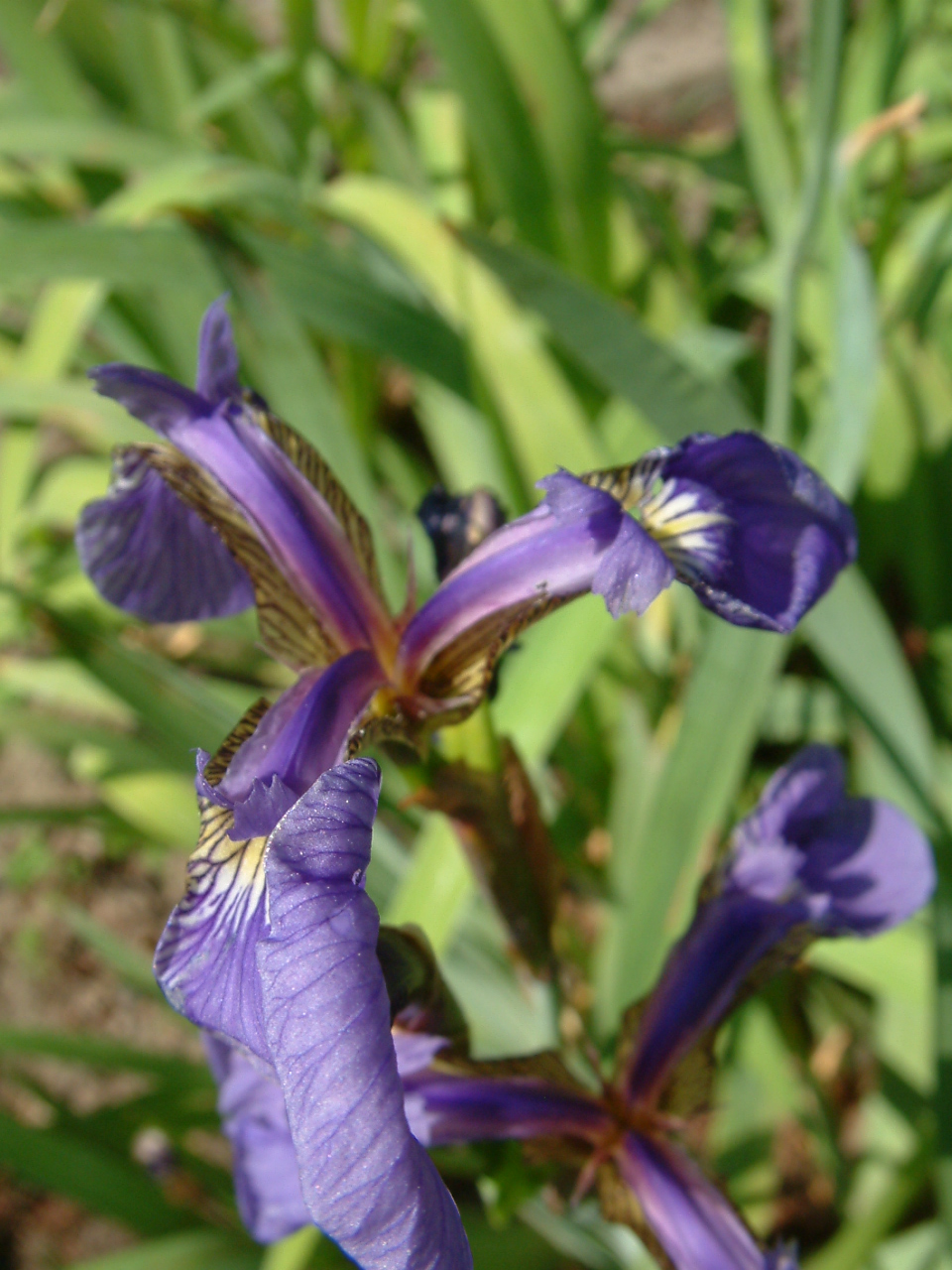
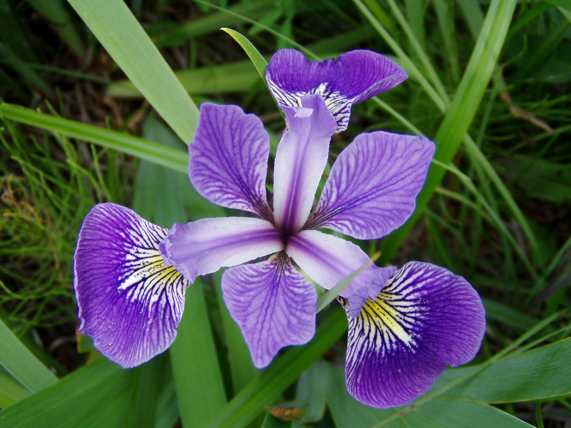
Here’s a picture of the three different Iris types:
# The Iris Setosa
from IPython.display import Image
url = 'http://upload.wikimedia.org/wikipedia/commons/5/56/Kosaciec_szczecinkowaty_Iris_setosa.jpg'
Image(url,width=300, height=300)
# The Iris Versicolor
from IPython.display import Image
url = 'http://upload.wikimedia.org/wikipedia/commons/4/41/Iris_versicolor_3.jpg'
Image(url,width=300, height=300)
# The Iris Virginica
from IPython.display import Image
url = 'http://upload.wikimedia.org/wikipedia/commons/9/9f/Iris_virginica.jpg'
Image(url,width=300, height=300)

The iris dataset contains measurements for 150 iris flowers from three different species.
The three classes in the Iris dataset:
Iris-setosa (n=50)
Iris-versicolor (n=50)
Iris-virginica (n=50)
The four features of the Iris dataset:
sepal length in cm
sepal width in cm
petal length in cm
petal width in cm
Get the data
Using seaborn to get the iris data.
import seaborn as sns
iris = sns.load_dataset('iris')
Let’s visualize the data!
Exploratory Data Analysis
Import some necessary libraries.
import pandas as pd
import matplotlib.pyplot as plt
%matplotlib inline
iris.head()
| sepal_length | sepal_width | petal_length | petal_width | species | |
|---|---|---|---|---|---|
| 0 | 5.1 | 3.5 | 1.4 | 0.2 | setosa |
| 1 | 4.9 | 3.0 | 1.4 | 0.2 | setosa |
| 2 | 4.7 | 3.2 | 1.3 | 0.2 | setosa |
| 3 | 4.6 | 3.1 | 1.5 | 0.2 | setosa |
| 4 | 5.0 | 3.6 | 1.4 | 0.2 | setosa |
Creating a pairplot of the dataset.
# Setosa is the most separable.
sns.pairplot(iris,hue='species',palette='Dark2')
<seaborn.axisgrid.PairGrid at 0x1b076aab700>
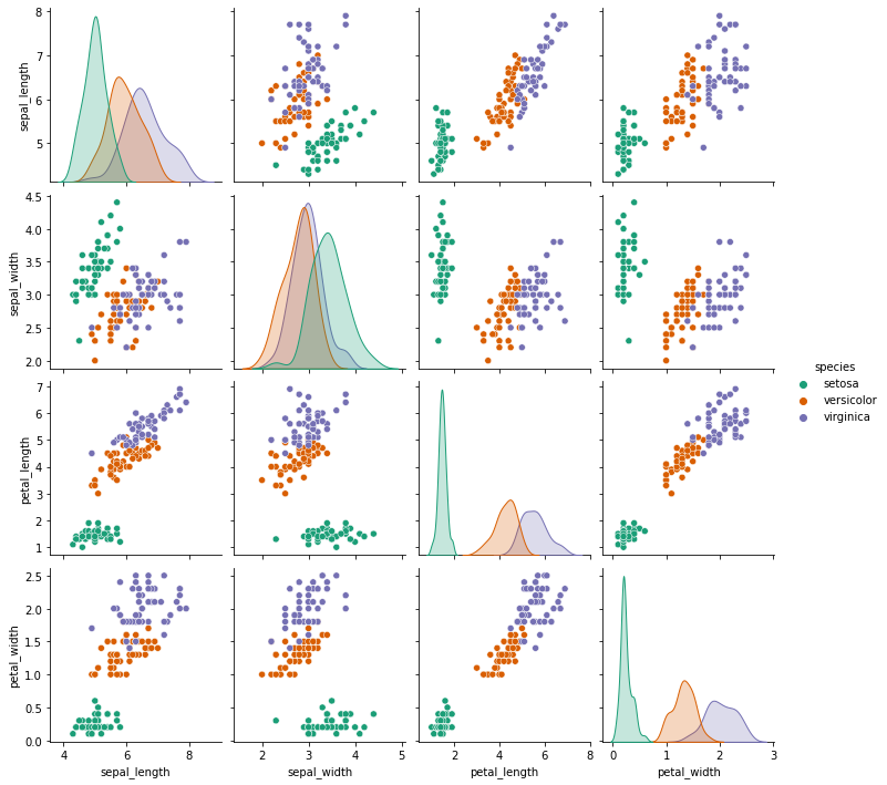
The species setosa seems to be the most separable here.
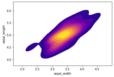
Creating a kde plot of sepal_length versus sepal width for setosa species of flower.
setosa = iris[iris['species']=='setosa']
sns.kdeplot( setosa['sepal_width'], setosa['sepal_length'],
                 cmap="plasma", shade=True, shade_lowest=False)
c:\Users\phull\python-venv\python39-venv\lib\site-packages\seaborn\_decorators.py:36: FutureWarning: Pass the following variable as a keyword arg: y. From version 0.12, the only valid positional argument will be `data`, and passing other arguments without an explicit keyword will result in an error or misinterpretation.
  warnings.warn(
c:\Users\phull\python-venv\python39-venv\lib\site-packages\seaborn\distributions.py:1718: UserWarning: `shade_lowest` is now deprecated in favor of `thresh`. Setting `thresh=0.05`, but please update your code.
  warnings.warn(msg, UserWarning)


<AxesSubplot:xlabel='sepal_width', ylabel='sepal_length'>
Train Test Split
Splitting our data into a training set and a testing set.
from sklearn.model_selection import train_test_split
X = iris.drop('species',axis=1)
y = iris['species']
X_train, X_test, y_train, y_test = train_test_split(X, y, test_size=0.30)
Train a Model
Now its time to train a Support Vector Machine Classifier.
Calling the SVC() model from sklearn and fitting the model to the training data.
from sklearn.svm import SVC
svc_model = SVC()
svc_model.fit(X_train,y_train)
SVC()
Model Evaluation
Now, we will get predictions from the model and create a confusion matrix and a classification report.
predictions = svc_model.predict(X_test)
from sklearn.metrics import classification_report,confusion_matrix
print(confusion_matrix(y_test,predictions))
[[18  0  0]
 [ 0 10  1]
 [ 0  2 14]]
print(classification_report(y_test,predictions))
              precision    recall  f1-score   support

      setosa       1.00      1.00      1.00        18
  versicolor       0.83      0.91      0.87        11
   virginica       0.93      0.88      0.90        16

    accuracy                           0.93        45
   macro avg       0.92      0.93      0.92        45
weighted avg       0.94      0.93      0.93        45
We can now notice that your model is pretty good! Let’s see if we can tune the parameters to try to get even better (unlikely, since the dataset is a bit small, but let’s try.)
Gridsearch Practice
Importing GridsearchCV from SciKit Learn.
from sklearn.model_selection import GridSearchCV
We will create a dictionary called param_grid and fill out some parameters for C and gamma.
param_grid = {'C': [0.1,1, 10, 100], 'gamma': [1,0.1,0.01,0.001]}
We will create a GridSearchCV object and fit it to the training data.
grid = GridSearchCV(SVC(),param_grid,refit=True,verbose=2)
grid.fit(X_train,y_train)
Fitting 5 folds for each of 16 candidates, totalling 80 fits
[CV] END .....................................C=0.1, gamma=1; total time=   0.0s
[CV] END .....................................C=0.1, gamma=1; total time=   0.0s
[CV] END .....................................C=0.1, gamma=1; total time=   0.0s
[CV] END .....................................C=0.1, gamma=1; total time=   0.0s
[CV] END .....................................C=0.1, gamma=1; total time=   0.0s
[CV] END ...................................C=0.1, gamma=0.1; total time=   0.0s
[CV] END ...................................C=0.1, gamma=0.1; total time=   0.0s
[CV] END ...................................C=0.1, gamma=0.1; total time=   0.0s
[CV] END ...................................C=0.1, gamma=0.1; total time=   0.0s
[CV] END ...................................C=0.1, gamma=0.1; total time=   0.0s
[CV] END ..................................C=0.1, gamma=0.01; total time=   0.0s
[CV] END ..................................C=0.1, gamma=0.01; total time=   0.0s
[CV] END ..................................C=0.1, gamma=0.01; total time=   0.0s
[CV] END ..................................C=0.1, gamma=0.01; total time=   0.0s
[CV] END ..................................C=0.1, gamma=0.01; total time=   0.0s
[CV] END .................................C=0.1, gamma=0.001; total time=   0.0s
[CV] END .................................C=0.1, gamma=0.001; total time=   0.0s
[CV] END .................................C=0.1, gamma=0.001; total time=   0.0s
[CV] END .................................C=0.1, gamma=0.001; total time=   0.0s
[CV] END .................................C=0.1, gamma=0.001; total time=   0.0s
[CV] END .......................................C=1, gamma=1; total time=   0.0s
[CV] END .......................................C=1, gamma=1; total time=   0.0s
[CV] END .......................................C=1, gamma=1; total time=   0.0s
[CV] END .......................................C=1, gamma=1; total time=   0.0s
[CV] END .......................................C=1, gamma=1; total time=   0.0s
[CV] END .....................................C=1, gamma=0.1; total time=   0.0s
[CV] END .....................................C=1, gamma=0.1; total time=   0.0s
[CV] END .....................................C=1, gamma=0.1; total time=   0.0s
[CV] END .....................................C=1, gamma=0.1; total time=   0.0s
[CV] END .....................................C=1, gamma=0.1; total time=   0.0s
[CV] END ....................................C=1, gamma=0.01; total time=   0.0s
[CV] END ....................................C=1, gamma=0.01; total time=   0.0s
[CV] END ....................................C=1, gamma=0.01; total time=   0.0s
[CV] END ....................................C=1, gamma=0.01; total time=   0.0s
[CV] END ....................................C=1, gamma=0.01; total time=   0.0s
[CV] END ...................................C=1, gamma=0.001; total time=   0.0s
[CV] END ...................................C=1, gamma=0.001; total time=   0.0s
[CV] END ...................................C=1, gamma=0.001; total time=   0.0s
[CV] END ...................................C=1, gamma=0.001; total time=   0.0s
[CV] END ...................................C=1, gamma=0.001; total time=   0.0s
[CV] END ......................................C=10, gamma=1; total time=   0.0s
[CV] END ......................................C=10, gamma=1; total time=   0.0s
[CV] END ......................................C=10, gamma=1; total time=   0.0s
[CV] END ......................................C=10, gamma=1; total time=   0.0s
[CV] END ......................................C=10, gamma=1; total time=   0.0s
[CV] END ....................................C=10, gamma=0.1; total time=   0.0s
[CV] END ....................................C=10, gamma=0.1; total time=   0.0s
[CV] END ....................................C=10, gamma=0.1; total time=   0.0s
[CV] END ....................................C=10, gamma=0.1; total time=   0.0s
[CV] END ....................................C=10, gamma=0.1; total time=   0.0s
[CV] END ...................................C=10, gamma=0.01; total time=   0.0s
[CV] END ...................................C=10, gamma=0.01; total time=   0.0s
[CV] END ...................................C=10, gamma=0.01; total time=   0.0s
[CV] END ...................................C=10, gamma=0.01; total time=   0.0s
[CV] END ...................................C=10, gamma=0.01; total time=   0.0s
[CV] END ..................................C=10, gamma=0.001; total time=   0.0s
[CV] END ..................................C=10, gamma=0.001; total time=   0.0s
[CV] END ..................................C=10, gamma=0.001; total time=   0.0s
[CV] END ..................................C=10, gamma=0.001; total time=   0.0s
[CV] END ..................................C=10, gamma=0.001; total time=   0.0s
[CV] END .....................................C=100, gamma=1; total time=   0.0s
[CV] END .....................................C=100, gamma=1; total time=   0.0s
[CV] END .....................................C=100, gamma=1; total time=   0.0s
[CV] END .....................................C=100, gamma=1; total time=   0.0s
[CV] END .....................................C=100, gamma=1; total time=   0.0s
[CV] END ...................................C=100, gamma=0.1; total time=   0.0s
[CV] END ...................................C=100, gamma=0.1; total time=   0.0s
[CV] END ...................................C=100, gamma=0.1; total time=   0.0s
[CV] END ...................................C=100, gamma=0.1; total time=   0.0s
[CV] END ...................................C=100, gamma=0.1; total time=   0.0s
[CV] END ..................................C=100, gamma=0.01; total time=   0.0s
[CV] END ..................................C=100, gamma=0.01; total time=   0.0s
[CV] END ..................................C=100, gamma=0.01; total time=   0.0s
[CV] END ..................................C=100, gamma=0.01; total time=   0.0s
[CV] END ..................................C=100, gamma=0.01; total time=   0.0s
[CV] END .................................C=100, gamma=0.001; total time=   0.0s
[CV] END .................................C=100, gamma=0.001; total time=   0.0s
[CV] END .................................C=100, gamma=0.001; total time=   0.0s
[CV] END .................................C=100, gamma=0.001; total time=   0.0s
[CV] END .................................C=100, gamma=0.001; total time=   0.0s


GridSearchCV(estimator=SVC(),
             param_grid={'C': [0.1, 1, 10, 100],
                         'gamma': [1, 0.1, 0.01, 0.001]},
             verbose=2)
Now using that grid model, we will create some predictions using the test set and create classification reports and confusion matrices for them.
grid_predictions = grid.predict(X_test)
print(confusion_matrix(y_test,grid_predictions))
[[18  0  0]
 [ 0 10  1]
 [ 0  0 16]]
print(classification_report(y_test,grid_predictions))
              precision    recall  f1-score   support

      setosa       1.00      1.00      1.00        18
  versicolor       1.00      0.91      0.95        11
   virginica       0.94      1.00      0.97        16

    accuracy                           0.98        45
   macro avg       0.98      0.97      0.97        45
weighted avg       0.98      0.98      0.98        45
We can see that we now have slightly better results.
There is basically just one point that is too noisey to grab and we don’t want to have an overfit model that would be able to grab that.